To the next level#
In this chapter we will explore aspects of the system that go beyond the simplest steps taken to build a relatively simple time series information system.
We will address:
performance issues regarding stored and computed series
working in depth with the task manager to build robust pipelines
how to efficiently organize the acquisition of a vast referential of raw series
good data architecture
Doing your own app using the Refinery#
The Refinery works well as a stand-alone tool, until you need to do any of the following:
data acquisition with dedicated tasks
new api points
new formula operators
The first item is by far the most common.
We propose to start with a skeleton app that we will call “myapp”. It structure is as follows (standard Python package app):
myapp
├── myapp
│   └── __init__.py
└── setup.py
The setup.py should be minimal and may contain this:
from setuptools import setup

setup(name='myapp',
   version='0.1.0',
   author='MyCorp',
   author_email='myself@mycorp.fr',
   description='Provide scrapers and tasks for my refinery',
   packages=['myapp'],
   install_requires=[
       'tshistory_refinery'
   ],
)
Data acquisition: a structured path#
In the chapter Pipelines : starting with injecting data we described an effective yet rudimentary strategy to implement data acquisition. The Refinery provides a tool to enable a better organization of this.
We will organize the scraping into two modules:
scrap_collection.py
scrap_config.py
The project application structure should be like this:
myapp/
├── myapp
│   ├── __init__.py
│   ├── scrap_collection.py
│   └── scrap_config.py
└── setup.py
The first one, scrap_collection, will host all our scraping functions. The second one, scrap_config, will provide a global scraping configuration for the application and of course use the scraping functions defined in the first one.
Let’s examine scrap_collection.py, restarting from the minimalistic scraper we wrote for the Pipelines : starting with injecting data.
import pandas as pd
from entsoe import EntsoePandasClient

def get_res_generation_forecast_entsoe(zone, fromdate, todate):
    metadata = {
        'source': 'entsoe',
        'country': zone,
        'category': 'res generation',
        'series-type': 'forecast'
    }
    try:
       df = EntsoePandasClient(api_key='apikey').query_wind_and_solar_forecast(
           zone,
           start=fromdate.tz_localize('Europe/Paris'),
           end=todate.tz_localize('Europe/Paris'),
       )
    except NoMatchingDataError:
       return pd.DataFrame(), metadata

    return df, metadata
Here are the differences with the previous one:
there is a zone parameter rather than a hard-coded ‘FR’ zone
we have a pair of fromdate and todate parameters
we don’t insert any data, we just return what we got (a time series and a dict to hold the metadata)
Let’s try to do something out of this immediately, this time we will populate the scrap_config module:
from functools import partial

from tshistory_refinery.scrap import (
    Scrap,
    Scrapers
)

from myapp.scrap_collection import get_res_generation_forecast_entsoe

SCRAPERS = Scrapers(
    Scrap(
       names={
           'power.prod.solar.fr.mwh.entsoe.fcst.h': 'Solar',
           'power.prod.windonshore.fr.mwh.entsoe.fcst.h': 'Wind Onshore'
       },
       func=partial(get_res_generation_forecast_entsoe, 'FR'),
       schedrule='0 5 * * * *',
       fromdate='(shifted (today) #:days -1)',
       todate='(shifted (today) #:days 7)',
       initialdate='(date "2015-1-1")'
    ),
    Scrap(
       names={
           'power.prod.solar.be.mwh.entsoe.fcst.h': 'Solar',
           'power.prod.windoffshore.be.mwh.entsoe.fcst.h': 'Wind Offshore',
           'power.prod.windonshore.be.mwh.entsoe.fcst.h': 'Wind Onshore'
       },
       func=partial(get_res_generation_forecast_entsoe, 'BE'),
       schedrule='0 5 * * * *',
       fromdate='(shifted (today) #:days -1)',
       todate='(shifted (today) #:days 7)',
       initialdate='(date "2015-1-1")'
    )
)
Let’s analyze this step by step, as there is a lot to unpack. As you can see at first glance, we can re-use our scraping functions for several uses and generate not just a pair of time series.
At the top-level, we define this big global variable named SCRAPERS, which will indeed contain the scrapers hold by the Scrapers object.
The Scrapers object will collect as many individual scrap configurations as needed (as coma separated objects). These are to be defined with the Scrap object.
Let’s look at the first one.
names={
    'power.prod.solar.fr.mwh.entsoe.fcst.h': 'Solar',
    'power.prod.windonshore.fr.mwh.entsoe.fcst.h': 'Wind Onshore'
}
The names in this case is a mapping from the final series name we want to the series names the scraping function will acquire (which is determined by the data provider, obtained through documentation … or looking at what comes at the end of their api). A scraping function can get one or many series.
func=partial(get_res_generation_forecast_entsoe, 'FR'),
This func parameter takes the scraping function. The signature of a scraping function must be of the form:
funcname(fromdate: pd.Timestamp, todate: pd.Timestamp)
That is: accept two positional parameters, fromdate and todate that must be a standard Python datetime or a Pandas timestamp (which must be timezone aware).
Our concrete scrap function in fact wants a first zone parameter, which is why, to be compliant, we give func a partial application of the scrap function with a concrete value (‘FR’). Hence we can re-use this technique for as many zones as upstream knows, and in our example with ‘BE’.
Next: the scheduling rule.
schedrule='0 5 * * * *',
This declares a cron rule with support for seconds. In this case we want it to run every hour of every day at minute 5 and second 0.
Then come the parameters for the horizon/time windows.
fromdate='(shifted (today) #:days -1)',
todate='(shifted (today) #:days 7)',
initialdate='(date "2015-1-1")'
initialdate specifies the first time stamp wanted for the series, fromdate and todate specify the time window for a given time series update.
Note
initialdate will be used once, when the series we want does not yet exist. The initial series history will be built from there.
The three timestamps are defined using a mini expression language comparable to that of the formula language. The tree primitives are:
today -> returns a timestamp as of today
date <datestr> -> builds a timestamp from a string
shifted <date> <delta> -> shifts a date by a given delta
Note
The <delta> for shifted is using a keyword notation. The available keywords are #:hours, #:days, #:weeks, #:months
In our case, since we are fetching a 7 days forecast, it is entirely reasonable to fetch data from yesterday to the next 7 days.
Well, having explained all of that, are we done yet ? Almost !
The last step will be about the final setup: we need the task system to be made aware of what we have done, and we will do it through a command line operation of the myapp application.
This entails having a cli (for “command line interface”) module in myapp, whose tree now looks like that:
myapp/
├── myapp
│   ├── cli.py
│   ├── __init__.py
│   ├── scrap_collection.py
│   └── scrap_config.py
└── setup.py
Let’s write the cli.py module contents:
import click

from tshistory.api import timeseries
from tshistory_refinery import cache

from myapp.scrap_config import SCRAPERS

@click.group()
def myapp():
    pass


@myapp.command(name='setup-scrapers')
def setup_scrapers():
    tsa = timeseries()
    engine = tsa.engine

    with cache.suspended_policies(engine):
        for scraper in SCRAPERS.scrapers.values():
            scraper.prepare_task(engine)


@myapp.command(name='first-imports')
def first_imports():
    tsa = timeseries()
    engine = tsa.engine
    for scr in SCRAPERS.scrapers.values():
        if scr.initialdate is not None:
            inputdata = scr.build_inputs('fetch_history')
            inputdata['reset'] = 0
            api.schedule(
                engine,
                'fetch_history',
                inputdata=inputdata,
                domain='scrapers'
            )
Pfew ! Ah, the ultimate step: inform the setup.py of the existence of command line operations. We add a keyword entry_point to the setup function inside, like this, after the install_requires keyword:
entry_points={
    'console_scripts': [
        'myapp=myapp.cli:myapp'
    ]
}
At installation time, this creates the myapp command line tool.
You can launch the initial import (to fetch the history from initialdate) with:
$ myapp first-imports
And then schedule the regular updates like that:
$ myapp setup-scrapers
Now we are really set.
Performance aspects: stored time series and formulas#
Managing a time series information system entails understanding a number of performance aspects. These are related to two main metrics:
data volumetry
amount of computation done
On data, the standard metric in the industry is the number of points. This is too imprecise however to understand read and write performance aspects, and also the storage density aspect of the Refinery.
The time series storage logical model is built on a tree of blocks. We basically store:
version entities, each pointing to an initial block
a tree of blocks of compressed points - up to 150 points can be lumped together into a single block
This model is unremarkable when it comes to store a lot of versions with few points. The worst case would be one version with one point. However it shines when it comes to handling large amounts of points with a reasonnable amount of versions; for instance, meteo forecasts which come three to four times per day with 15 days worth of hourly forecasts. Density storage in these circumstances is excellent.
On computation (for the formulas), the effort is directly proportional to:
the amount of data involved,
the complexity of involved operations.
A simple resample formula is cheap and can be computed on the fly with a reasonably small overhead. But in a developped time series information system, formulas of formulas exist and it is possible to have a very deep level of formulas made of formulas until one hits the ground of stored time series, hence increasing latency, sometimes very noticeably.
When the performance of complex formulas becomes an issue, it is possible to set up a regularly refreshed materialized view, or cache, which will make operational use of the complex formulas manageable again. This aspect is addressed in the next chapter.
Formulas: when to use a cache/materialized view#
There exist two main scenarios leading to use a formula cache:
formulas with autotrophic operators
very complex (computation intensive) formulas
The first case relates to custom operators made to act as a proxy for another time series repository. In the Refinery we have two builtin operators that are autotrophic: series and constant. These operators do not transform data, they are a source of data.
Writing an autotrophic operator is a viable option if (and only if):
the remote source provides an API that can be adapted for the needs of the Refinery,
the latency of the remote source remains reasonnably low.
Even in the best case, such an operator can have some nasty performance characteristics from the point of view of the remote source: a new load at arbitrary times that interferes with the load as initially designed. Caching formulas made with such operators can help smooth out the load and establish good relationships with the upstream source.
The case of computationally intensive formulas is simple: we need to have access to a freshly computed version of the formula.
We will explain how to do this in the next chapter.
How to cache formulas#
Theory#
Caching a formula is not a matter of pushing a button and get a working cache ! That would be too easy … The very nature of versioned time series forces us to think about how to do it properly.
Let’s have a look at a series from the point of view of the two time axis:
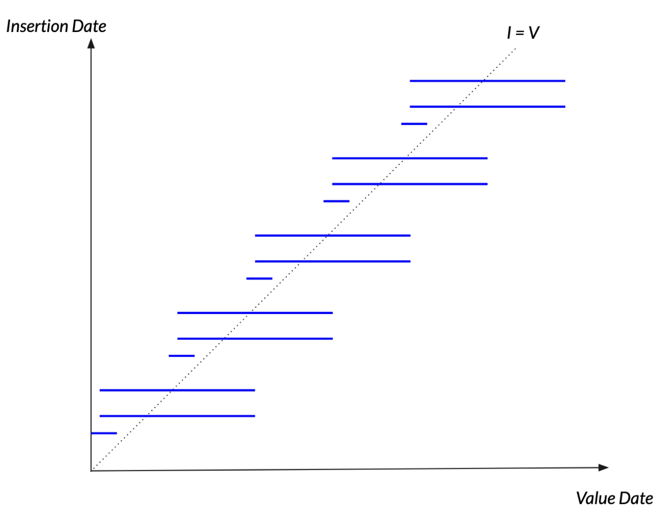
The blue lines represent new points along the value date axis. We have new blue lines for each version. On this graph, we should realize that we are seeing elements of a forecast, for many points go into the future.
Understanding the relationship between the value dates (horizontal axis) and insertion dates (vertical axis), and their regularities, is key to set up a working cache policy.
So let’s define immediately the notion of cache policy. It is characterized by:
an initial revision date (or insertion date)
a revision rule for the advancement of the revision dates
a time window associated with the current revision date (look_before / look_after)
Note
We use the terms revision date and insertion date as pure synonyms.
If we apply these notions to the time series seen above, we can propose a cache policy like the following:
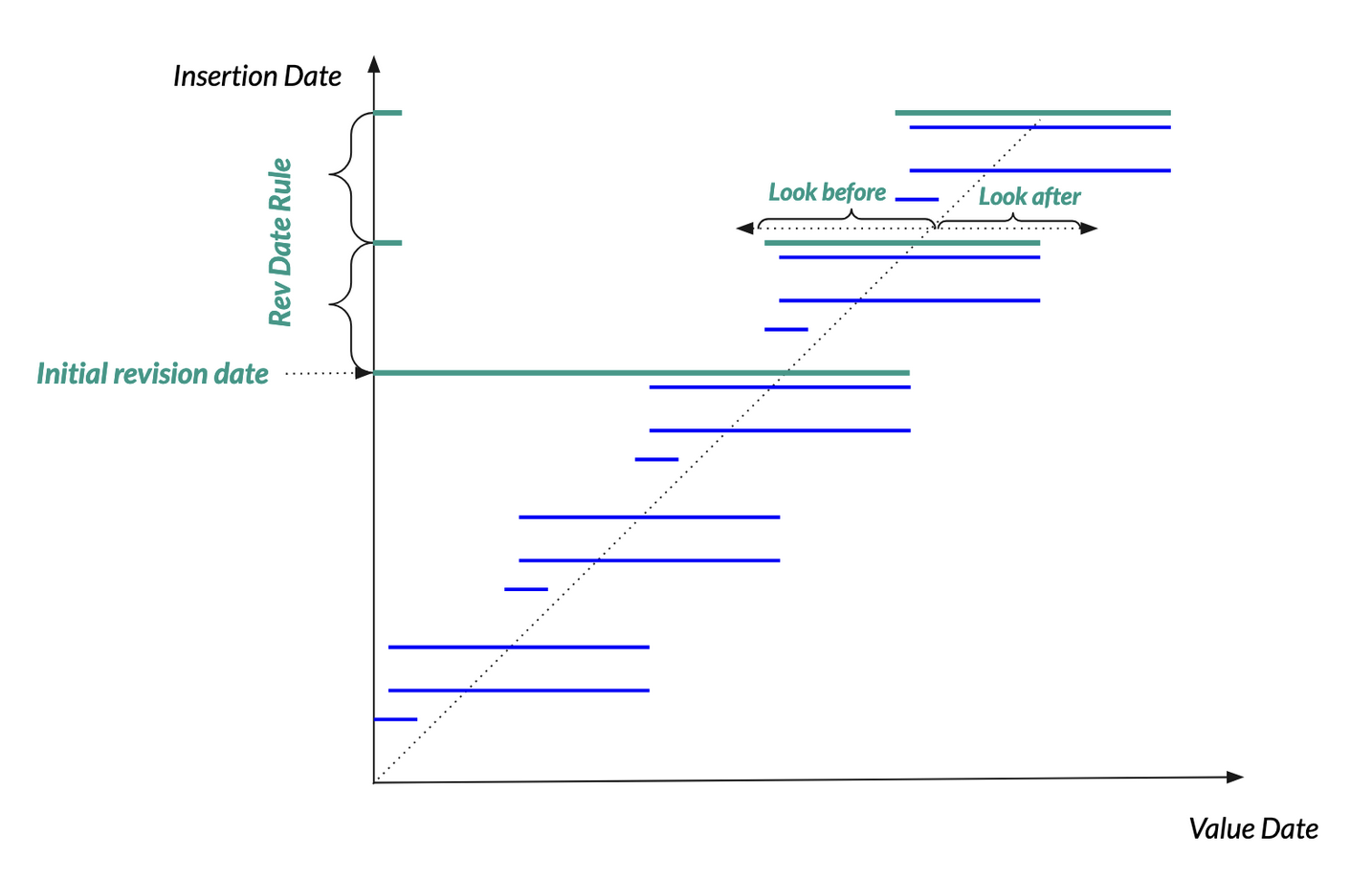
The optimal cache policy will exploit our knowledge of the time series temporality aspects.
So with the initial revision date we put an arbitrary point in the past before which the time series formula has in effect no materialized counterpart. This is because old enough versions get more rarely accessed as time moves on. There has to be a compromise between time and space. Revisions before the initial revision date will be computed on the fly.
The revision rule should match the expected refresh frequency of the time series. Since a formula’s insertion dates is naturally the union of all the underlying components, it makes sense to think about this expected refresh frequency: we want to avoid getting spurious revisions, and we need to have all the relevant (business wise) ones.
Lastly, the time window allows querying the system with limited bounds, so as to minimize the load when building the cache. For instance, using the full horizon all the time could have nasty performance implications.
It must be configured so as to:
permit catching possible updates to the observed domain,
guarantee the lossless ingestion of the predictive part of the curve.
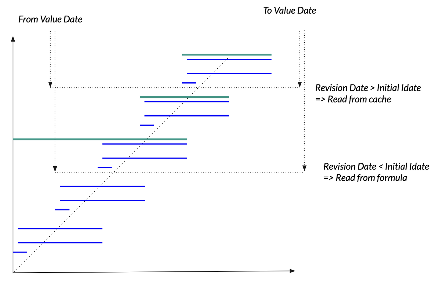
Now let’s observe how the presence of a formula cache affects the reading of such a time series:
Note
There is another aspect not mentioned in the above drawing: when the time delta between now and the latest cache revision date is two “ticks” behind according to the revision date rule (that is: potentially stale), we do actually use the formula to get the result.
Practice#
The Web UI provides a whole section dedicated to the maintenance of cache policies.
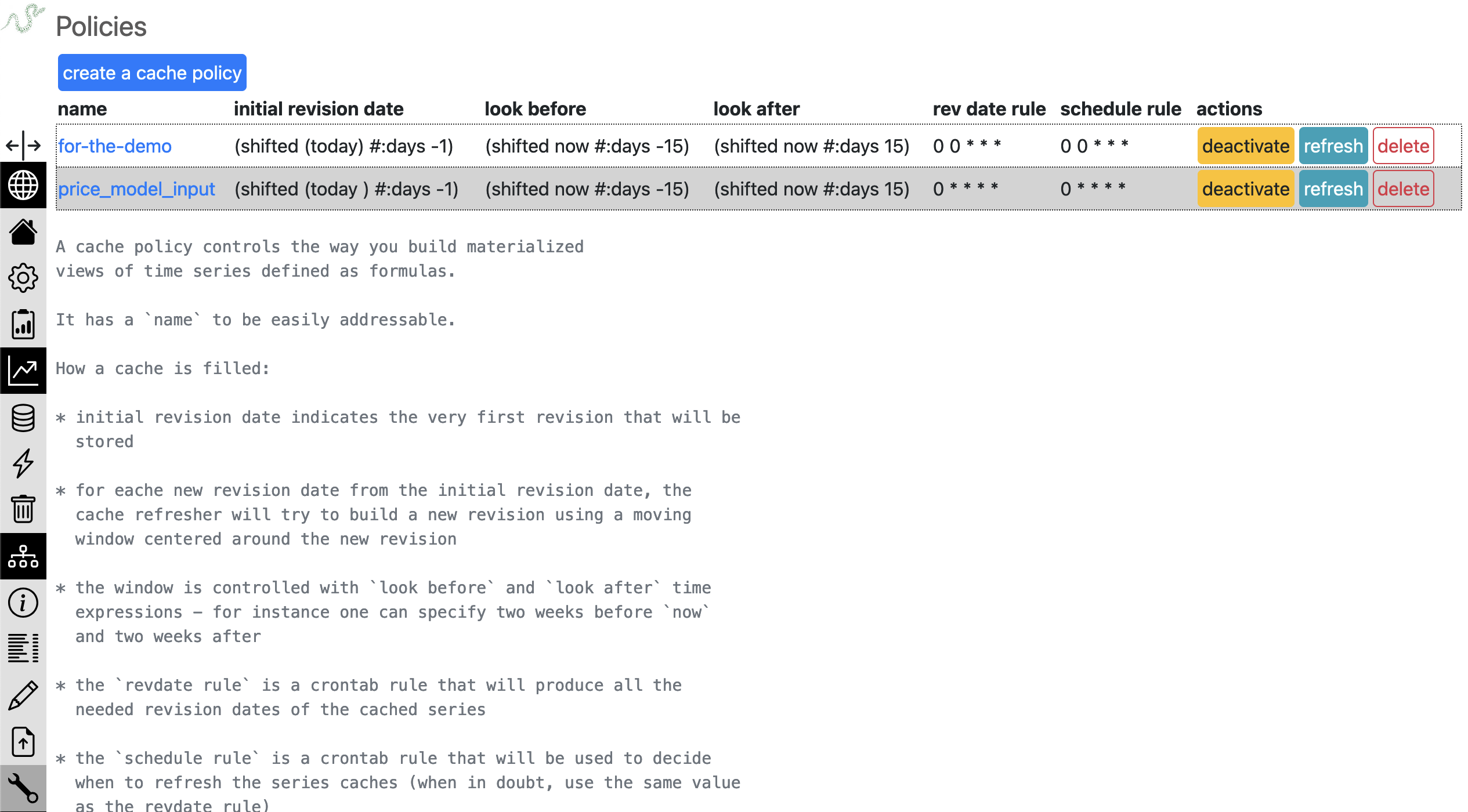
The list at the top shows the existing cache policies. We can create or edit a policy, leading us to the following policy creation form:
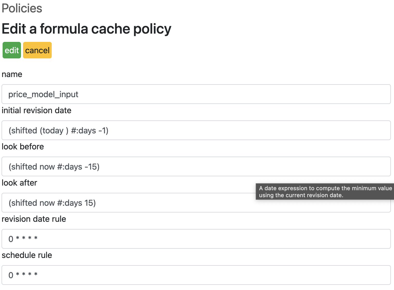
You need to give it a clear name. A cache policy will be associated with as many formulas as you want, which makes sense provided they have the same common time and data patterns, as explained in the previous chapter.
The fields initial revision date, look before and look after all use the same Lisp-like mini language. Here’s the list of available functions:
today -> produces a timestamp as of now
shifted <timestamp> -> takes keywords minutes, hours, weeks and months to shift the input timestamp by the required time delta
date <datestr> -> turns the date string input into an actual timestamp
The look before and look after will generally use a now variable rather than today. When the cache is being updated, this variable will be valued with the corresponding revision date.
Examples:

(today)
(shifted (today) #:weeks -1)
(date "2024-1-1")
(shifted now #:days 15)
The revision date rule and schedule rule must be described according to the cron syntax.
When in doubt, you should assign the same value to schedule rule and to revision date rule. It sometimes makes sense to schedule the actual cache update using a different rule than the revision date rule (to smooth out the strain on server resources for instance).
When the cache policy has been created, it can be of course edited again, activated (otherwise nothing happens) or deleted.

The last step is managing the series associated with the policy. One gets there by clicking the policy name in the list.
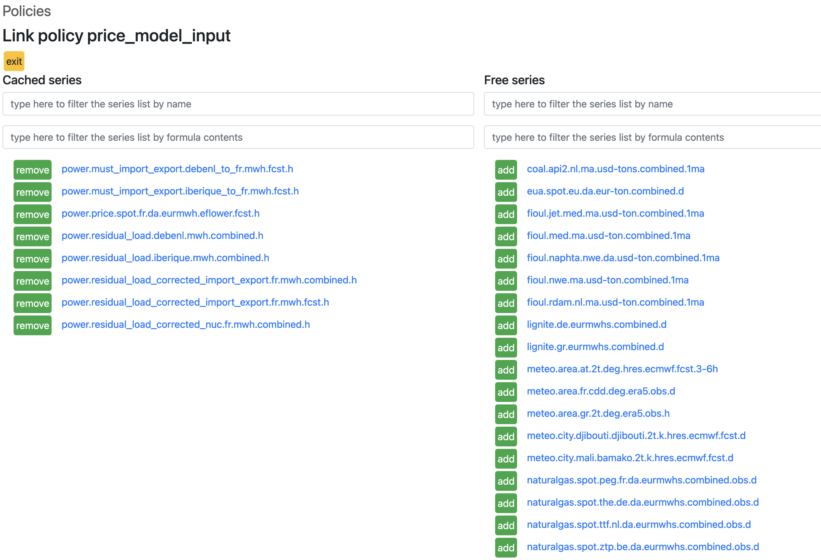
Tasks system: how to organize and schedule tasks#
In this chapter we will survey the basics of the tasks system, how to write and run tasks, and the best ways to organize them.
The built-in tasks system allows to organize, schedule and run tasks for (non limitative list):
data acquisition
data monitoring
running models
Note
The builtin tasks manager is not exclusive of any other tasks manager you want to use. Dask, Airflow or other such tools are fine in and by themselves and can certainly be used along with the Refinery if their workflows are more compelling for your specific use cases.
Basics: operations, domains, inputs, tasks#
Let’s review the most important concepts.
A task is the execution of an operation. An operation is a Python function that will run as a task. Here’s an example:
from rework.api import task

@task
def hello(task):
    with task.capturelogs(std=True):
        print('Hello')
Let’s examine what’s there:
the operation is marked by the task decorator
it must be a one parameter function, whose parameter is a task object.
the task object provides a number of methods, such as capturelogs
the capturelogs method accepts an std parameter, which when True turns the output of the print function into logs; capturelogs records the logs from any logger within its context
Such a task will also run in the “default” domain. A domain is basically a label allowing to group operations. It certainly makes sense to e.g. have separate domains such as models and scrapers. The Web UI permits filtering based on domains.
from datetime import timedelta
from rework.api import task
import rework.io as rio
from tshistory.api import timeseries

from eflower.models import run_co2_forecast

@task(domain='models',
      inputs=(
          rio.string('zone', required=True),
          rio.moment('fromdate', default='(today)'),
          rio.number('startoffset')
      ),
      timeout=timedelta(hours=2)
)
def co2_model(task):
    inputs = task.input
    tsa = timeseries()
    with task.capturelogs(std=True):
        run_co2_forecast(
            tsa,
            zone=inputs['zone'],
            fromdate=inputs['fromdate'],
            start_offset=inputs.get('start_offset', 0)
        )
In this example, we define an operation to run a model, in a dedicated models domain, with typed inputs. Here we see that the task decorator accepts:
a domain parameter (string),
an inputs parameter (tuple of rework.io entities), to specify inputs with Web UI support (in the Launchers tab)
As can be seen in the code, the inputs come as an attribute of the task object, and is a dictionary.
Registering and running tasks#
Operations defined in a Python module are not magically known from the system: an explicit single registration step has to be performed.
Let’s see the command line way, assuming you have all your operations definitions in a tasks.py module:
$ rework register-operations my_refinery myproject/tasks.py
registered 2 new operation (0 already known)
The dual operation is available.
$ rework unregister-operation refinery helloworld
preparing de-registration of:
delete helloworld default /home/aurelien/tasks.py 10.211.55.4
really remove those? [y/N]: y
delete helloworld default /home/aurelien/tasks.py 10.211.55.4
To have a fully working system, the last step is running a monitor for the models domain. A monitor is a program that manages a pool of workers for a given domain.
$ rework monitor my_refinery --maxruns 2 --maxworkers 4 --minworkers 1 --domain models --vacuum P4D
Let’s unpack this:
minworkers specifies the min amount of running workers in the pool,
maxworkers specifies the absolute maximum of workers,
maxruns indicates how many tasks a worker is allowed to run before being shut down (and eventually replaced),
domain specifies the domain,
vacuum defines the retention duration of tasks in the done state, using the iso 8601 durations notation.
A good organisation#
The notion of domains permits to group operations together. There can be a semantic aspect to the grouping (let’s not mix models and scrapers) and performance aspects, since each domain will be associated with a monitor, which has its own settings (configuration of the workers pool and tasks retention duration).
Out of the box, the Refinery uses two domains: timeseries and scrapers.
timeseries is used to run the formula cache operations,
scrapers is used to run the scraping operations.
You of course are encouraged to have your own domains. Reasonnable proposals seen in the field are:
models to run your models,
high-frequency to run operations that really want to run often, like e.g. every minute (hence they will clog the tasks list and you want to be able to easily filter them out)
Don’t forget to run at least one monitor for each domain !
Note
It is possible to run several monitors for one given domain. Hypothetical scenario: your computing units are too small to run all operations of a given domain in paralell, so you build several ones, using a Python environment with the same dependency versions on several machines.
Last point: if you have e.g. models but with incompatible requirements (typically in terms of versions), you can put them in different domains, managed by monitors living in different Python environments.
Tasks: using the Web UI#
The task manager provides a convenient Web UI to provide the users a dependable view of the state of the system. The UI provides a number of tabbed views and a couple of direct views. Let’s walk through them.
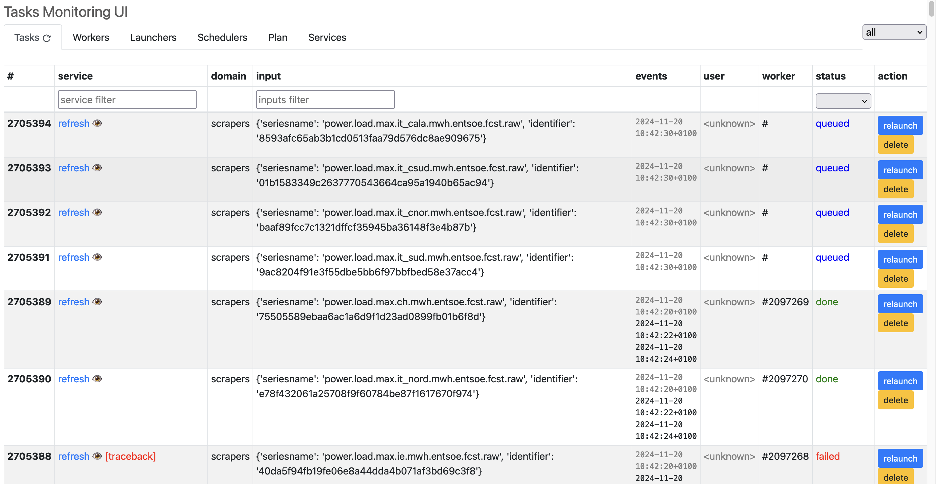
The tasks list is the first thing to be seen when we land on the tasks manager views. It provides a direct access to the tasks (status, inputs, domain, logs) and a few actions, in inverse chronological order (most recent at the top).
By default, the complete list is not loaded. By scrolling downwards, one gets new lazily loaded items.
The actions available on tasks are:
relaunch (can be useful when a task has been aborted for some reason)
delete (to unclutter the list)
abort (available only on running tasks)
Note
For the filters (on the service, inputs and status columns) to work appropriately, having everything loaded at once is more convenient. The “Tasks” tab provides an action to force load all known tasks in the list.
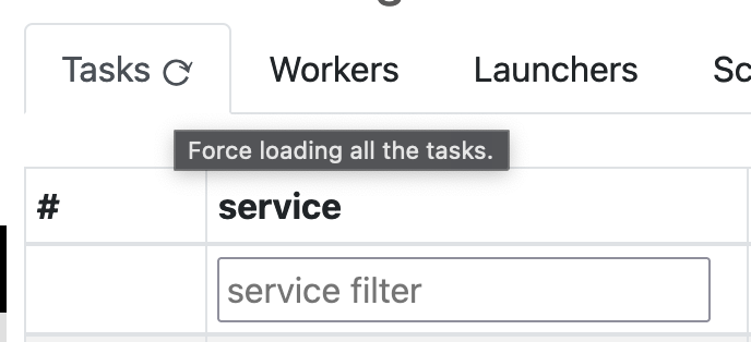
Clicking on the curved arrow symbol will force load all tasks.
By clicking on a task item (blue link on the operation name), one jumps to the task log (available if it is running or done).

For failed tasks, clicking on the traceback link in red opens the task back trace.
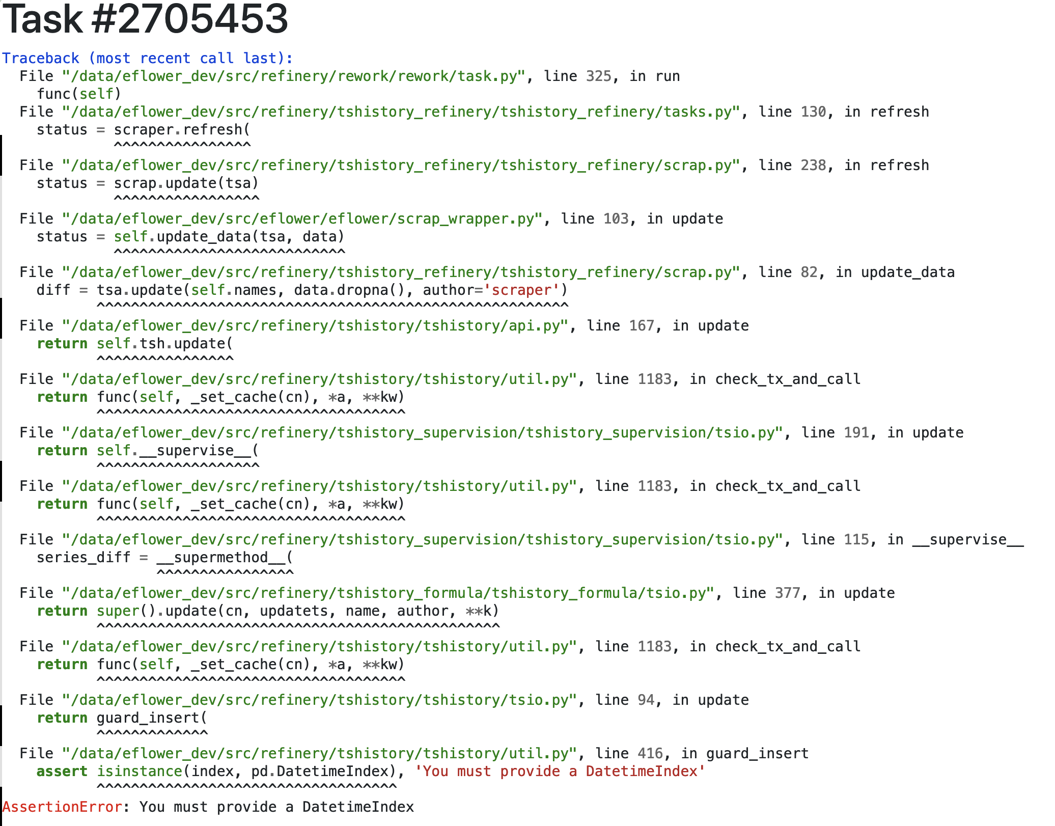
These two last views are important tools to understand what is going on with your tasks.
The next tab shows the monitors status. As we have seen, monitors provides workers for a given domain. We can see their state (their status is updated using a dead-man switch scheme) and their active workers.
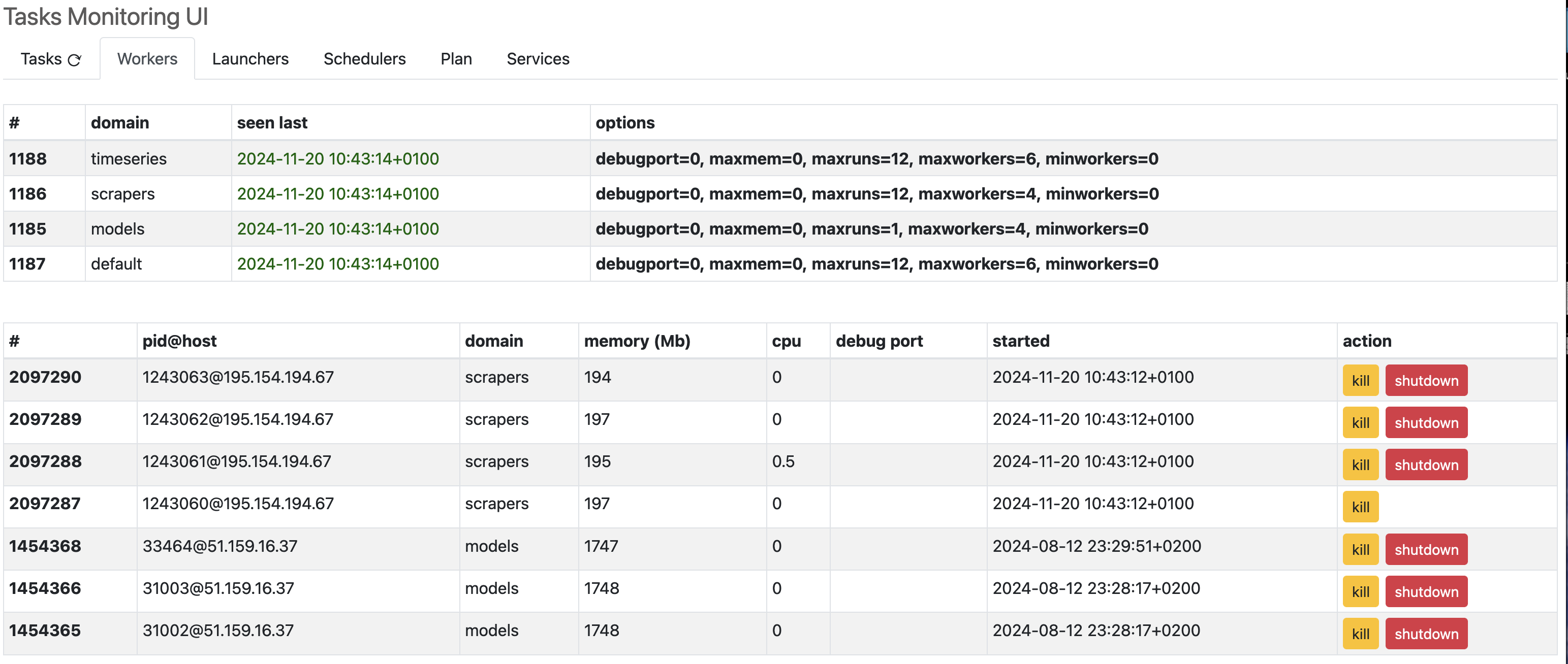
It is possible to ask for a shutdown (the worker will disappear after finishing its current task), or a kill (the worker is stopped and removed immediately).
The “Launchers” tab provides a zone to manually launch a task, either through a “launch now” action (when there are no inputs) or through an “open form” dialog to allow inputing the relevant operations parameters before launching.
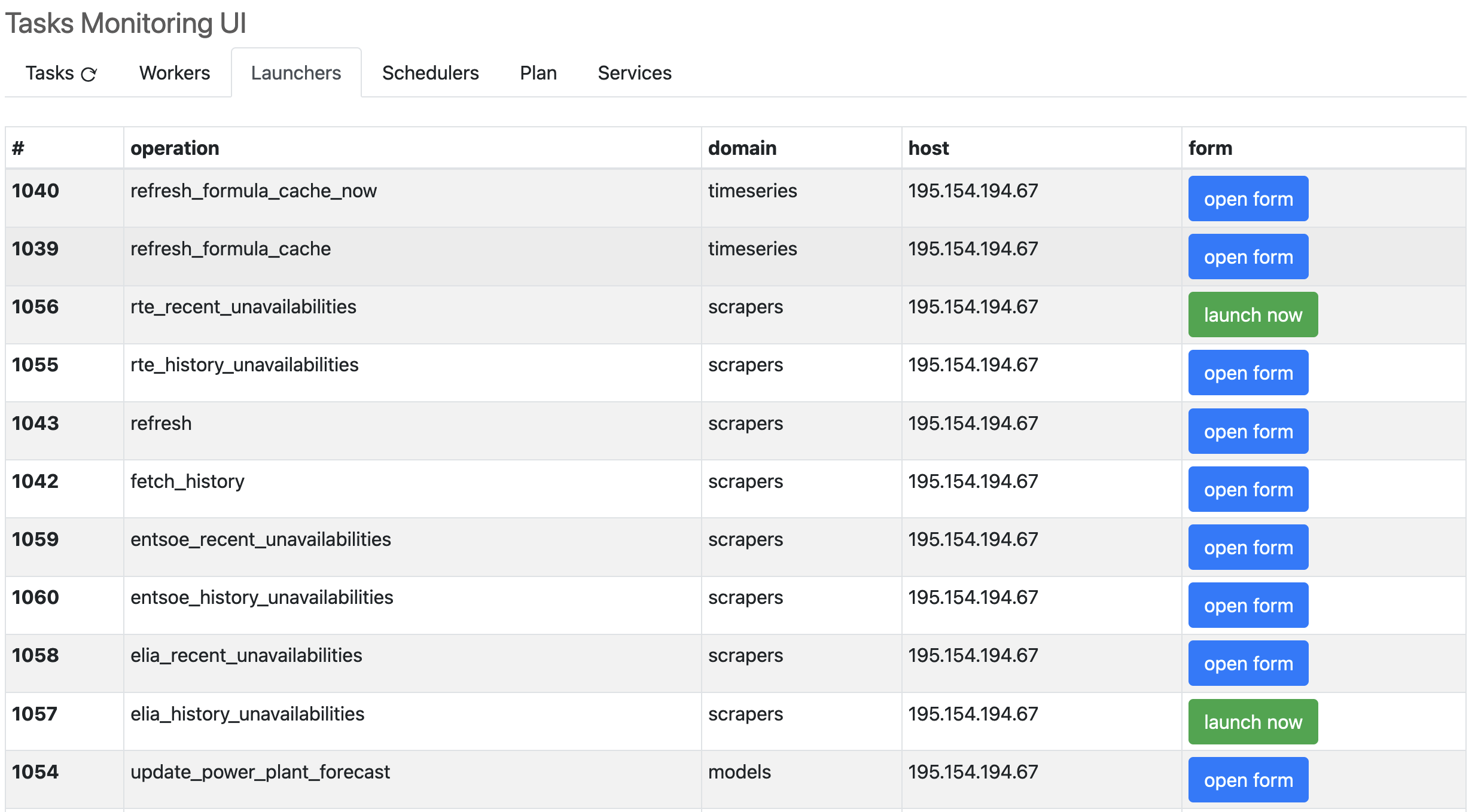
Note
For the tasks to be directly launchable from the Launchers tab, their declaration must contain an inputs declaration (even with an empty tuple if you need none). Only with this formalism can the UI know it can present actions, and which ones, to the end-user.
The “Schedulers” tab lists all pre-scheduled tasks with their inputs and schedule rule, also allowing to do an immediate launch if needed.
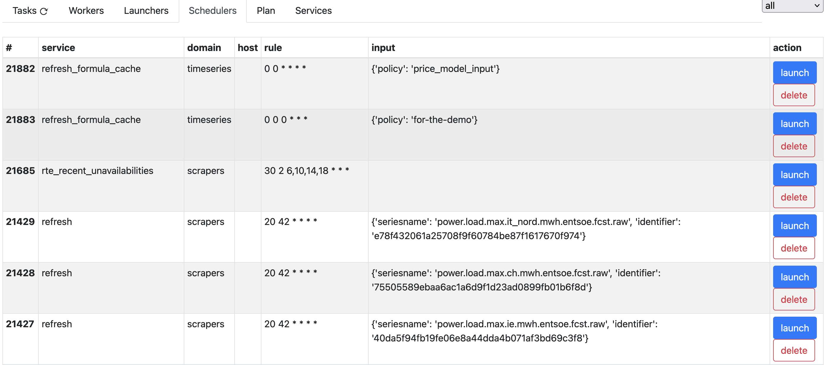
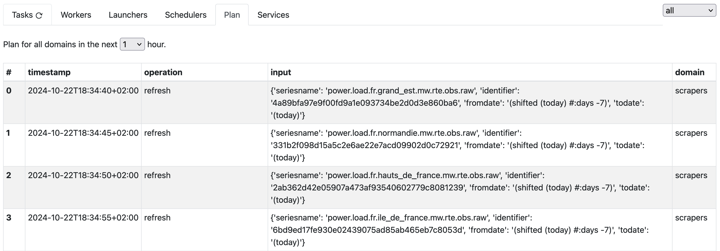
The “Plan” tab shows what tasks (amongst those that are pre-scheduled) are going to fire, and at which moment, with their inputs, in the next few hours.
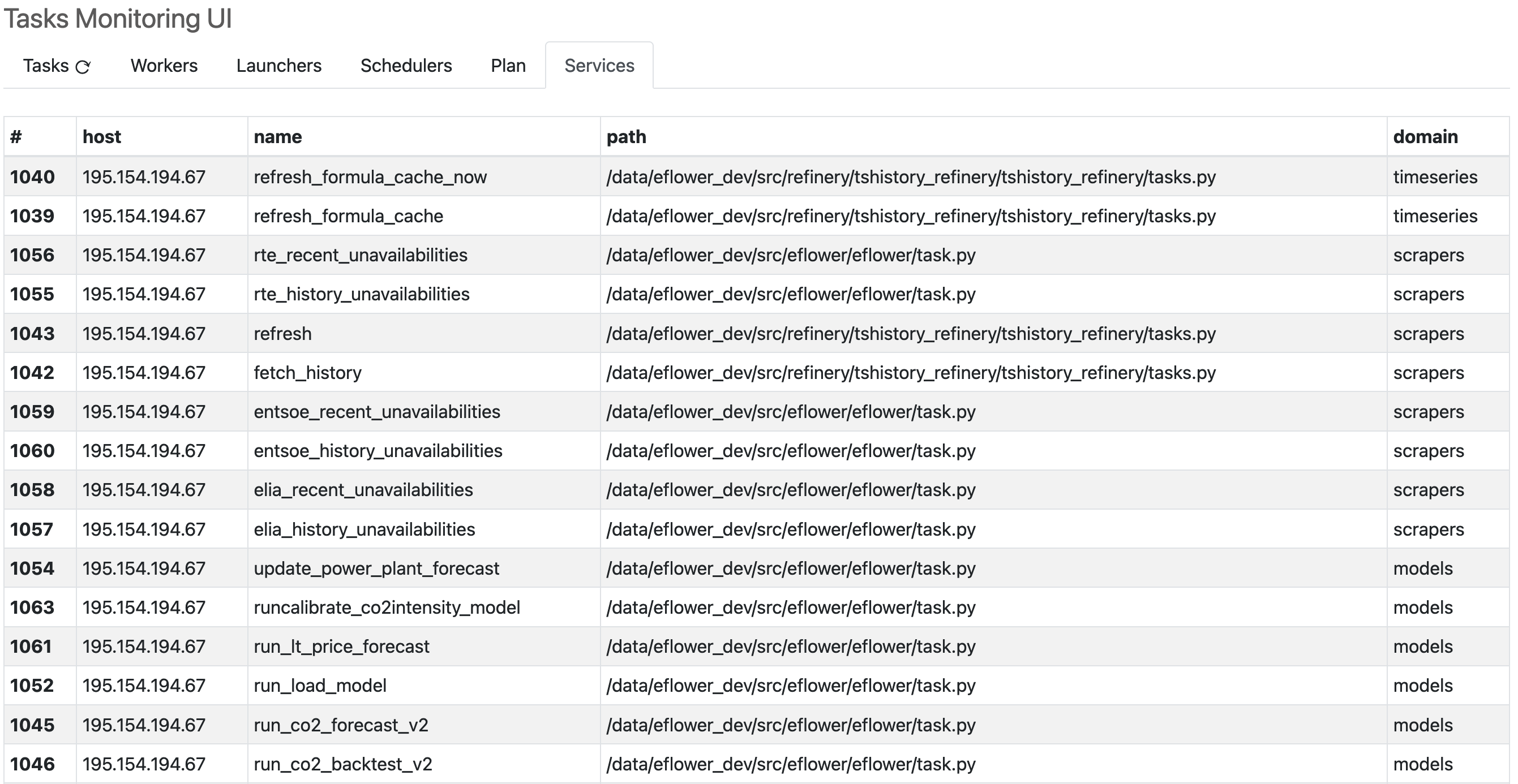
The final “Services” tab lists all the operations, notably with their host and file system path.
Data architecture at scale: putting the Data Mesh to work#
For a number of reasons, it may be a good idea to run not just one instance of the Refinery, but several interconnected in a data mesh, and also have some of them interconnected. Let’s see some of the reasons:
team/topics diversity
data architecture choice
Making teams work together#
Energy commodity companies sometimes have significant trading desks with a sizeable amount of analysts, data scientists and IT quant people working together. These people have different specialties, scopes and requirements. One useful way to address their specific needs is to provide a number of Refineries, each dedicated to a specific group.
Let’s imagine an hypothetical department where you have analysts working on oil, coal, power and gas. The “power” people are interested into renewables, nuclear, hydro and fossil fuel plants, and “gas” people are interested in piped and lng gas, also in storages and terminals. You get the idea. All these people work on production and demand models, which entails having access to meteorological data (forecasts).
Putting everyone’s data into one big data lake, I mean a big Refinery instance would quickly turn it into a data swamp, I mean a terrible mess. What we can propose is that each theme gets its own Refinery instance. You would have power, gas, oil, meteo, etc. refineries.
But then, the power and gas people (for instance) would need access to the meteo data, for their forecasting models need meteo forecasts as inputs.
Also the management would like to have a trans-commodity view of their position and get something consolidated: we can give them a Refinery connected to all others (and very little, if any, data of its own).
In this setup, each team can focus on its own needs, and delegate what they don’t master to other teams. The important power team (of several analysts and data scientists) would rely on the meteo team to provide them with the relevant solar and wind forecasts. The gas people modelling the demand would also ask the meteorologists about temperature forecasts in some places of interest.
So each teams gets its own Refinery, which means a local “data governance”, naming convention, workflows, models, etc. and at the same time data is easily shared cross-teams.
The Medallion Architecture#
This architecture was invented to address the needs of Data Lake users and avoid the Data Swamp syndrome which can afflict them. In the medallion architecture, we have layers of data. Each layer corresponds to a data state (“bronze” for raw data, “silver” holds the pre-processed raw data and “gold” contains completely curated data fit for consumption by everyone).
This layered approach can be an inspiration for the organization of Refineries, with:
a “bronze” Refinery holding data as scraped from the upstream providers (in versioned time series form of course), including missing data, outliers, changing granularities discontinuities and other warts,
a “silver” Refinery holding mostly formulas based on the “bronze” level, where we do proper resampling, basic outliers elimination, bogus data overrides, basic aggregations and data assemblies (using e.g. the add and priority formula operators) - this layer knows “bronze” which its use as a secondary, read-only source
a “gold” Refinery used as inputs for the models and also storing their outputs, providing data for dashboard and any other decision support tools - this layer uses the “silver” curated time series
Note
In a Data Lake, we have a hodge-podge of raw (json, xml) data, non relational and relational (with normalized and dernormalized relations) data bases, and so on; this complexity cries for the application of a doctrine such as the Medallion Architecture. On the other hand, Refineries are light-weight and provide structure from the start, but still the layering idea has some merit and could be put to work for instances with either a lot of time series at each levels, or a lot of stake holders at each level, to provide more overall clarity and better data governance.