Create a time series information system#

In the basics chapter, we’ve seen how to use a number of essential building blocks.

Building on this knowledge, we want to address a more ambitious goal: how to write a coherent, well curated time series information system.

We will start from the acquisition of time series data. There are some challenges there and we will address the most common.

Once we have a complete “primary data” set, made of raw time series, we will start the process of building the refined series that we can use:

as input for models
as input for high-level analysis (e.g. fundamental economic analysis)
as a basis for complex dashboards and decision support systems

At the end of this chapter, you will master all fundamental aspects of building a complete system.

Pipelines : starting with injecting data#

Data acquisition is the first step.

Let’s start with a simple example, in which we will get forecasts for renewable production in France. We will use a ready made open source client to get data from the ENTSO-E data repository. ENTSO-E itself exposes data for free in the context of the UE power markets.

 import pandas as pd
 from entsoe.exceptions import NoMatchingDataError
 from entsoe import EntsoePandasClient
 from tshistory.api import timeseries

 def get_res_generation_forecast_entsoe():
     fromdate = pd.to_datetime('today') - pd.Timedelta(1, 'd')
     todate = pd.to_datetime('today') + pd.Timedelta(7, 'd')
     try:
         df = EntsoePandasClient(api_key='apikey').query_wind_and_solar_forecast(
             'FR',
             start=fromdate.tz_localize('Europe/Paris'),
             end=todate.tz_localize('Europe/Paris'),
         )
     except NoMatchingDataError:
         return

     name_map = {
         'Solar': 'power.prod.solar.fr.mwh.entsoe.fcst.h',
         'Wind Onshore': 'power.prod.windonshore.fr.mwh.entsoe.fcst.h'
     }

     tsa = timeseries()
     for col, name in name_map.items():
         tsa.update(name, df[col], author='entsoe-scraper')

Such a scraping function, put into a Python script, could then be scheduled to be run at periodic moments of the day to continuously feed the time series repository; for instance using cron on Linux or at on Windows.

This is a bare-bones solution, which unsurprinsinly is largely used in the industry. Some prefer to use sophisticated and refined task schedulers such as Apache AirFlow, for the additional capacities it provides. Later in this document we will show how to use the Refinery integrated task manager to set up powerful data acquisition pipelines.

Now, let’s back to our scraping function and examine what it does in detail.

fromdate = pd.to_datetime('today') - pd.Timedelta(1, 'd')
todate = pd.to_datetime('today') + pd.Timedelta(7, 'd')

Here we start by defining the time window for the data to be fetched. Since it is about forecasts, a window from yesterday to next week is reasonnable.

try:
    df = EntsoePandasClient(api_key='apikey').query_wind_and_solar_forecast(
        'FR',
        start=fromdate.tz_localize('Europe/Paris'),
        end=todate.tz_localize('Europe/Paris'),
    )
except NoMatchingDataError:
    return

Next, we fetch the data using the ENTSO-E client dedicated method. We provide the zone and the time window. On error we exit immediately.

name_map = {
    'Solar': 'power.prod.solar.fr.mwh.entsoe.fcst.h',
    'Wind Onshore': 'power.prod.windonshore.fr.mwh.entsoe.fcst.h'
}

The resulting data frame may have several columns. We know (by reading the documentation) that in our case (zone FR) we will have two columns. We construct a mapping from these column names to the series names we want to have. It is very important to have a good naming convention (in our case we indicate: nature of the flux, type of production, zone, provenance of the data, nature of the data - forecast is not observed nor a nomination - and finally the expected granularity).

tsa = timeseries()
for col, name in name_map.items():
    tsa.update(name, df[col], 'entsoe-scraper')

We create the time series refinery api object and then do an update of the series.

This is one of the simplest thing we can do to acquire data.

Note

This however is a bit ad-hoc and lacks separation of concerns:

acquisition and injection happens in the same place
the horizon/time window handling is hard-coded
there is no handling of metadata, and we won’t know easily the provenance of the acquired data
we hard-coded the zone and time window

In the chapter on advanced topics we will propose a more structured way to organize this and address the issues listed above.

Using the task manager#

To have this scraping function running, we need a scheduler. We propose a small tour of the integrated task manager.

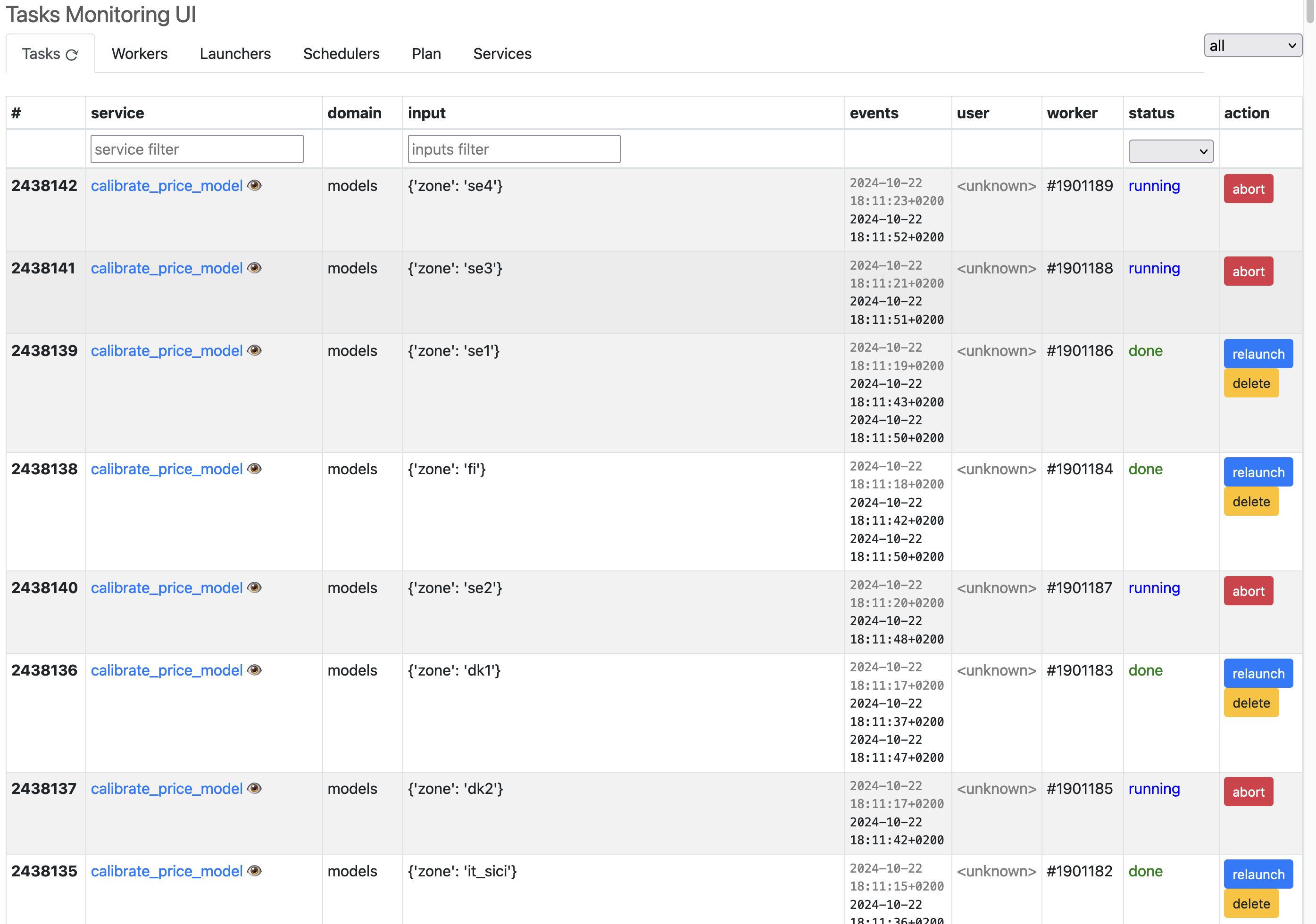
Here is how it looks:

The first tab shows the list of tasks that are either:

queued
running
done (or failed or aborted)

Each task shown there is defined by a Python function and an input.

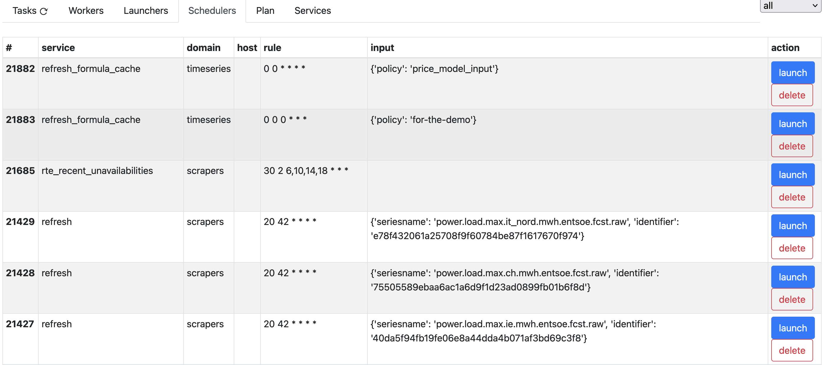
The tasks do not run at arbitrary times: the scheduler tab shows how tasks will be scheduled.

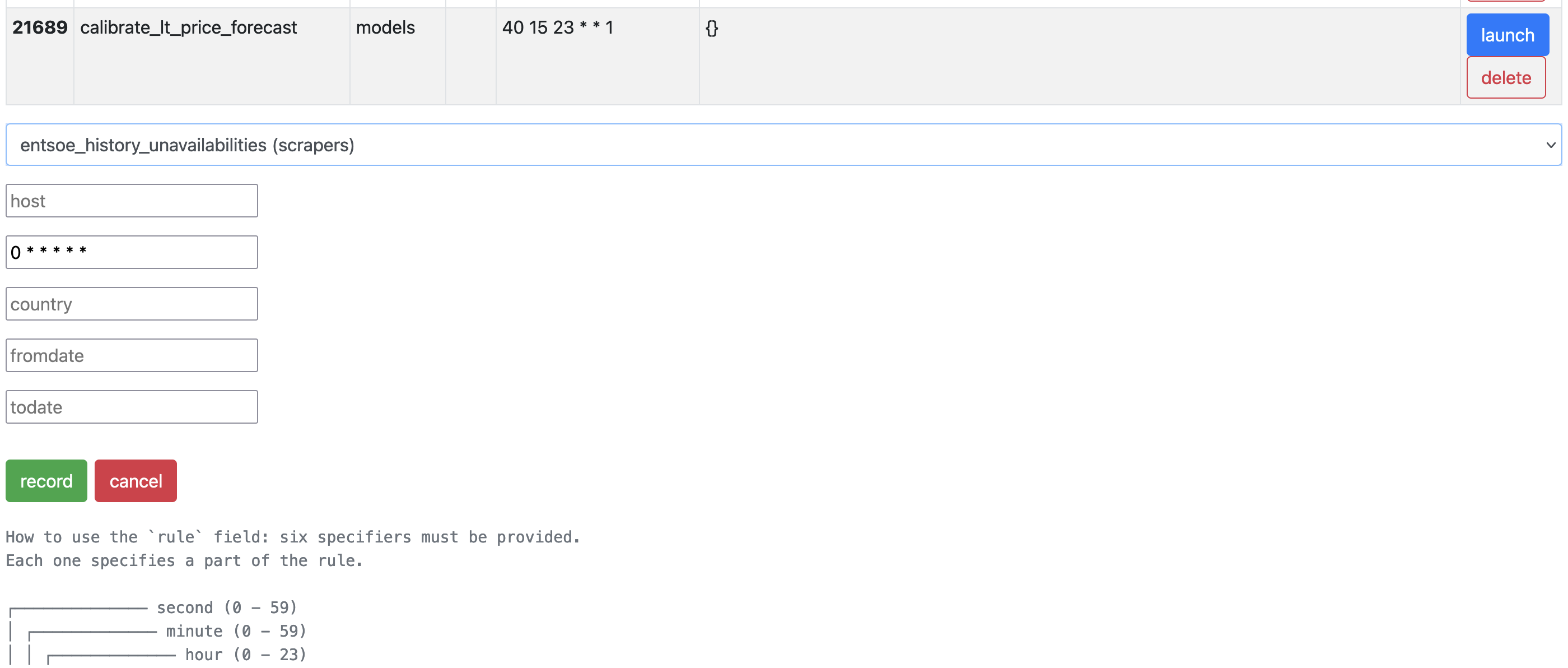
The most important column in this view is scheduler: it exposes a scheduling rule whose syntax obeys the laws of the cron tool.

Note

The cron-like notation used for the scheduler actually supports rules down to the seconds, hence the 6 fields. The rules for seconds are the same as for minutes.

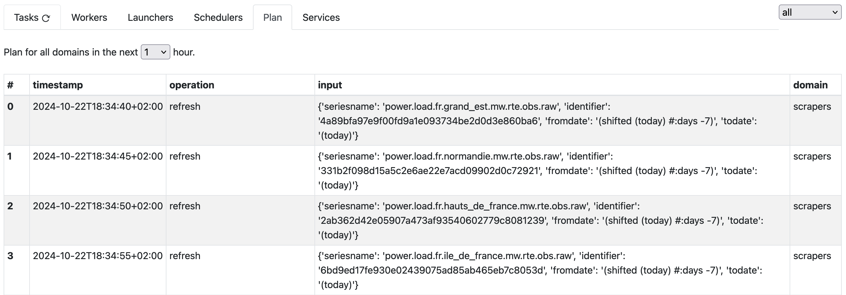
The plan tab shows the tasks that will be scheduled in the next 1 hour.

This is all what we need to finely control our scraping activities. Now let’s look at how to land it there !

Writing and using scrapers for primary series#

We need to define a task:

from rework.api import task

@task
def scrap_res_generation_forecast_entsoe(task):
    get_res_generation_forecast_entsoe()

This is the strict minimum. For comfort, we can do a bit more, as in this version:

from rework.api import task

@task
def scrap_res_generation_forecast_entsoe(task):
    with task.capturelogs(std=True):
        get_res_generation_forecast_entsoe()
        print('Success !')

The capturelogs context manager will make sure the task system will collect, when the task runs, all the logs. The std parameter allows to also capture everything coming out of the print function. Very handy to trace and follow what is going on.

Note

The @task decorator supports various options not shown there. You will find a complete description of its capabilities in the chapter on the task manager. Notable options are domain and timeout.

Having written this, we must register the task. We’ll do like this (assuming you have put the code above in a Python module named mytasks.py):

$ rework register-operations refinery mytasks.py

Now, this is ready to run. You can go to the Launchers tab and start your task immediately, or go the Schedulers tab and organize its scheduling rule (there is an action for that at the bottom of the page).

When the task is appearing in the tasks list, you can click on its name to get to see the logs. It may look like that:

Building formulas on top to get curated series#

With the basics of data injection in place, we can now turn to the construction of the time series we actually want. It is certainly possible to write computing functions and put them into tasks like we did for data acquisition, but we propose a nicer way to do it. Indeed, arbitrary Python code is very powerful but it has downsides:

it is unsafe (you just can’t accept random python code from your analysts on the server side of operations), so you need a lengthy and costly validation workflow to have it deployed
it is (by default at least) not type-safe
it takes quite some time to learn to do it properly
it is not easily reusable or composable nor shareable (still possible but it takes a lot of learning to do it properly)
seeing the computation may be difficult and auditing it can become very complicated quickly

We have a solution to these issues:

use a very simple safe domain specific expression language to do the computations
call this a “formula language” (like for Excel), suitable for non-programmers
do the computations on the fly (by default: doing materialized computations remains possible, especially for performance reasons)
provide a vast array of composable primitive operators (all of pandas can be made available if necessary, plus more)
define computed time series from this base, that will a) belong to the time series referential and b) look like a stored time series for all intents and purposes (for the read operations at least)

By limiting the computation power, we actually gain more powers !

In the basics chapter we learnt how to create and use formulas. Let see how to apply this knowledge to build our time series information system.

A first step would be normalization. Its purpose is to adress the following (non-exhaustive) list of questions :

do the raw series have the needed granularities ?
are these granularities actually constant ? If we perform our analysis on e.g. hourly time series, can we make sure our computation will start from hourly series (without throwing away data) ?
are the raw data using the units we want to work with (e.g. MWh, euros) ?
are the raw series complete or do we need to combine some together to get a coherent picture ?
how do we manage outliers ?

So we can write formulas that provides a first layer of transformation.

Assuming we scrap the series power.price.spot.at.da.eurmwh.entsoe.obs.raw from ENTSO-E; that series flipped from hourly to 15-minutely granularity in october 22, and later reverted back to hourly. We want to prevent this discontinuity. So let’s write a simple formula:

(resample "power.price.spot.at.da.eurmwh.entsoe.obs.raw" "h")

Using the register_formula api call, we create power.price.spot.at.da.eurmwh.entsoe.obs.h:

tsa.register_formula(
    'power.price.spot.at.da.eurmwh.entsoe.obs.h',
    '(resample "power.price.spot.at.da.eurmwh.entsoe.obs.raw" "h")'
)

Meteo temperature time series from ERA5 are provided in Kelvin. A conversion to Celsius could be useful:

(+ -273.15 (series "meteo.area.ch.2t.k.era5.obs.h"))

Completeness: it is not uncommon to have raw series describing the same fundamental data, while being different in a subtle way. For instance, one source has a long history but its update frequency on recent data is spotty; and then you find another source with less history depth but more stringent update baheviour. Let’s combine them into a well-behaved series:

(priority
    (series "power.price.spot.dk1.da.eurmwh.entsoe.obs.h")
    (series "power.price.spot.dk1.da.eurmwh.epex.obs.h"))

The priority operator is immensely helpful there. It wil take the points of the first series if there are any - barring that, the points of the second series are selected.

Another situation for priority, with 3 series this time: some flux have observed data, nominated data, and forecasted data. We can combined these three into a single series:

(priority
    (series "gas.flow.ne.dunkirk.gassco.msmd.obs")
    (series "gas.flow.ne.dunkirk.gassco.msmd.nom")
    (series "gas.flow.ne.dunkirk.gassco.msmd.fcst")

Outliers: this is a complex topic, which is highly dependent on the nature of the data. There exists simple situations where bluntly removing obviously bogus values works. To do that, we can use the clip operator.

(clip (series "this-series-cannot-be-negative") #:min 0)

Feeding a model with series, getting the output in the system, with the task manager#

Overview#

In this section, we demonstrate how to implement a model in the timeseries refinery. As an example, we use a simple linear regression, to emphasize the interaction with the refinery. A modelisation process will alternate between two main phases: calibration and forecast.

The calibration process needs input and output data and produces calibration parameters.

The forecast process needs input data and calibration parameters and produces output estimation.

The calibration parameters are stored in base, which allows to decouple the two operations. Moreover, the evolution of these parameters is valuable information, hence we want to store them without deleting the previous ones. For this purpose, we use the dbcache package shipped with tshistory_refinery.

This package proposes 3 types of API: - a cache with an associated lifetime - a key-value store - a versioned key-value store

In this case we are using the later (called vkvstore).

Initialisation#

We initialize in the postgres database a new namespace dedicated to our models parameters.

In order to to that one has to type the following command:

$ dbcache init-db  <dburi> --namespace calibration

Here are now the necessary python functions. Necessary imports:

import json

import pandas as pd
from sklearn.linear_model import LinearRegression
from sklearn.metrics import r2_score

from tshistory.api import timeseries
from dbcache.api import vkvstore

Calibration per se:

def calibrate(tsa):
    # input
    x = tsa.get('meteo.area.fr.2t.k.era5.obs.h')
    # output
    y = tsa.get('power.load.fr.mwh.entsoe.obs.h')
    x.name = 'x'
    y.name = 'y'
    common = pd.concat([x, y], axis=1, join='inner')

    predictor = LinearRegression(n_jobs=-1)
    predictor.fit(X=common[['x']], y=common[['y']])
    slope = predictor.coef_[0][0]
    intercept = predictor.intercept_[0]

    # we want to store some indicator of fitness:
    r2 = r2_score(
        common[['y']],
        predictor.predict(common[['x']])
    )
    # we prepare the serialization of the calibration parameters
    # the pickle method should be avoided for archive purpose
    results = {
        'slope': slope,
        'intercept': intercept,
        'r2': r2,
    }

    return results

Save the calibration parameters:

def save_coefficients(tsa, results):
    store = vkvstore(tsa.uri, 'calibration')
    # vkvstore use string as keys and bstring as values
    json.dumps(results)
    store.set(
        'linear-calibration-key',
        json.dumps(results).encode('utf-8')
    )

Note

Note the “calibration” string in the vkvstore api which references the string used as namespace in the dbcache init-db command.

Now for the forecasting, we need to load the saved parameters:

def load_coefficients(tsa):
    store = vkvstore(tsa.uri, 'calibration')
    stored = store.get('linear-calibration-key')
    return json.loads(stored.decode('utf-8'))

And finally read the input data, apply the model on it and store the results as a timeseries:

def forecast(tsa, coefficients):
    x = tsa.get('meteo.area.fr.2t.k.era5.obs.h')
    predicted = x * coefficients['slope'] + coefficients['intercept']
    name = 'power.load.fr.mwh.linear.fcst.h'
    tsa.update(
        name,
        predicted,
        'linear-model'
    )

We can now assemble these operations in two distincts tasks:

@task(inputs=(), domain='models')
def linear_calibration(task):
    with task.capturelogs(std=True):
        tsa = timeseries()
        results = calibrate(tsa)
        save_coefficients(tsa, results)

@task(inputs=(), domain='models')
def linear_forecast(task):
    with task.capturelogs(std=True):
        tsa = timeseries()
        coefficients = load_coefficients(tsa)
        forecast(tsa, coefficients)

This tasks can then be scheduled, accordingly to your calibration/forecasting rules.